Plot survey indices

Usage

plot_si(fit, type = "model_fit", base_size = 8)

Arguments

fit: A gadget fit object. See g3_fit.
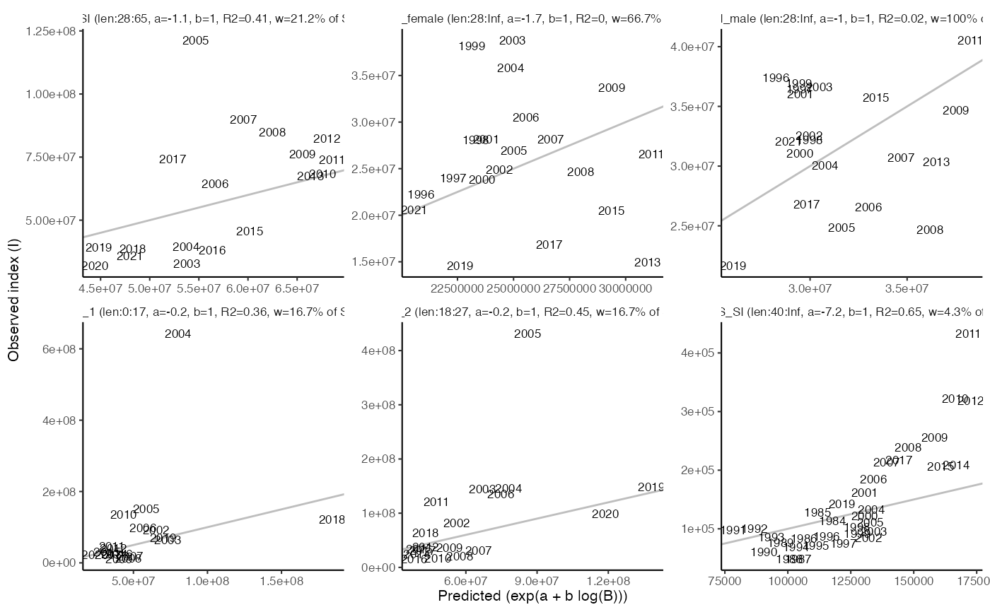
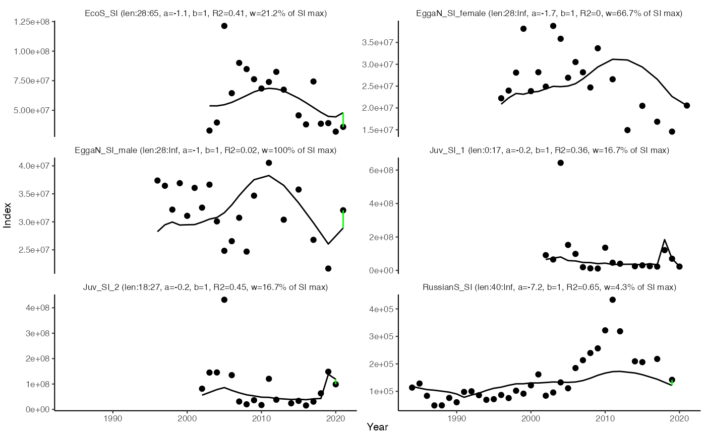
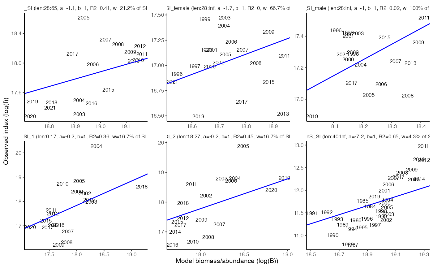
type: Character specifying the plot type: "model_fit" plots the model fit to survey index data by year, "regression" plots regression lines together with logarithms of model biomass/abundance and observed index values, and "scatter" produces a scatter plot for the predicted and observed index using the same values than in "model_fit". See details.
base_size: Base size parameter for ggplot. See ggtheme.

Value

A ggplot object.

Details

Relationship between a survey index (I) and model biomass or abundance (B) over a defined length range is expressed as \(I = e^a B^b\), where \(e^a\) is the catchability (also called q) and b the stock size dependent catchability (see type = "model_fit"). Whether I is compared to model biomass or abundance, depends on the units of I (i.e. column name of the data object; "number" -> abundance, "weight" -> biomass). The survey index I is called "observed" in the figure, and "predicted" is derived as \(exp(a + b \; log(B))\). The a and b can be visualized using a log-linear formula \(log(I) = a + b \; log(B)\) (see type = "regression"; log-linear regressions shown using blue lines). The coefficient of determination \(R^2\) is calculated using this regression. To compare the observed and predicted values in the model fit plot, use type = "scatter". The grey line represents a diagonal line with a slope of 1 and intercept of 0 (i.e. \(I = B\), \(a = 0\), \(b = 1\)).

Examples

data(fit)
plot_si(fit)

plot_si(fit, type = "regression")

plot_si(fit, type = "scatter")