Gadget3 array-handling utilities — array

Tools to make munging array reports easier

g3_array_agg(
        ar,
        margins = NULL,
        agg = c(
            "sum",
            "length_mean", "length_sd",
            "predator_length_mean", "predator_length_sd" ),
        opt_time_split = !("time" %in% margins || "time" %in% ...names()),
        opt_length_midlen = FALSE,
        ... )

g3_array_combine(
        arrays,
        agg = sum,
        init_val = 0 )

g3_array_plot(
        ar,
        legend = "topright" )

Arguments

ar: Input array, e.g. dstart_fish__num from a model report, or list of arrays
arrays: List of input arrays, can be a nested list as generated by cons in g3_quota_assess
margins: dimension names to include in the final array, e.g. c("age", "year") to generate a report by-year & age. If NULL, no aggregation is done
agg: Function or character. Function to use when aggregating, or name of one of the built-in functions
init_val: The initial value to use when combining arrays
opt_time_split: Boolean, should we split up "time" into separate "year" & "step" dimensions?
opt_length_midlen: Boolean, should we convert "length"
legend: Location of legend, passed to legend's x parameter
...: Filters to apply to any dimension, including "year" / "step" if opt_time_split is TRUE. e.g. length = 40, age = 5, step = 1

Details

g3_array_agg allows you to both filter & aggregate an array at the same time.

Specifying a filter in ... is simplfied in comparison to a regular R subset:

You can give the dimensions in any order
Values are always interpreted, age = 3 will be interpreted as "age3", not the third age.

For particular dimensions we have extra helpers:

age: Numeric ages e.g. age = 5 are converted to "age5", as generated by gadget3
length: Numeric lengths will pick a value within groups, e.g. with lengths "10:20", "20:30", length = 15 will pick the smaller lengthgroup

g3_array_combine generates the union of 2 disjoint arrays, so you can combine aggregated output from an immature and mature stock for example.

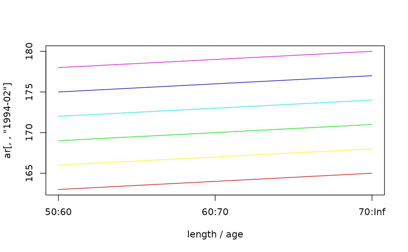
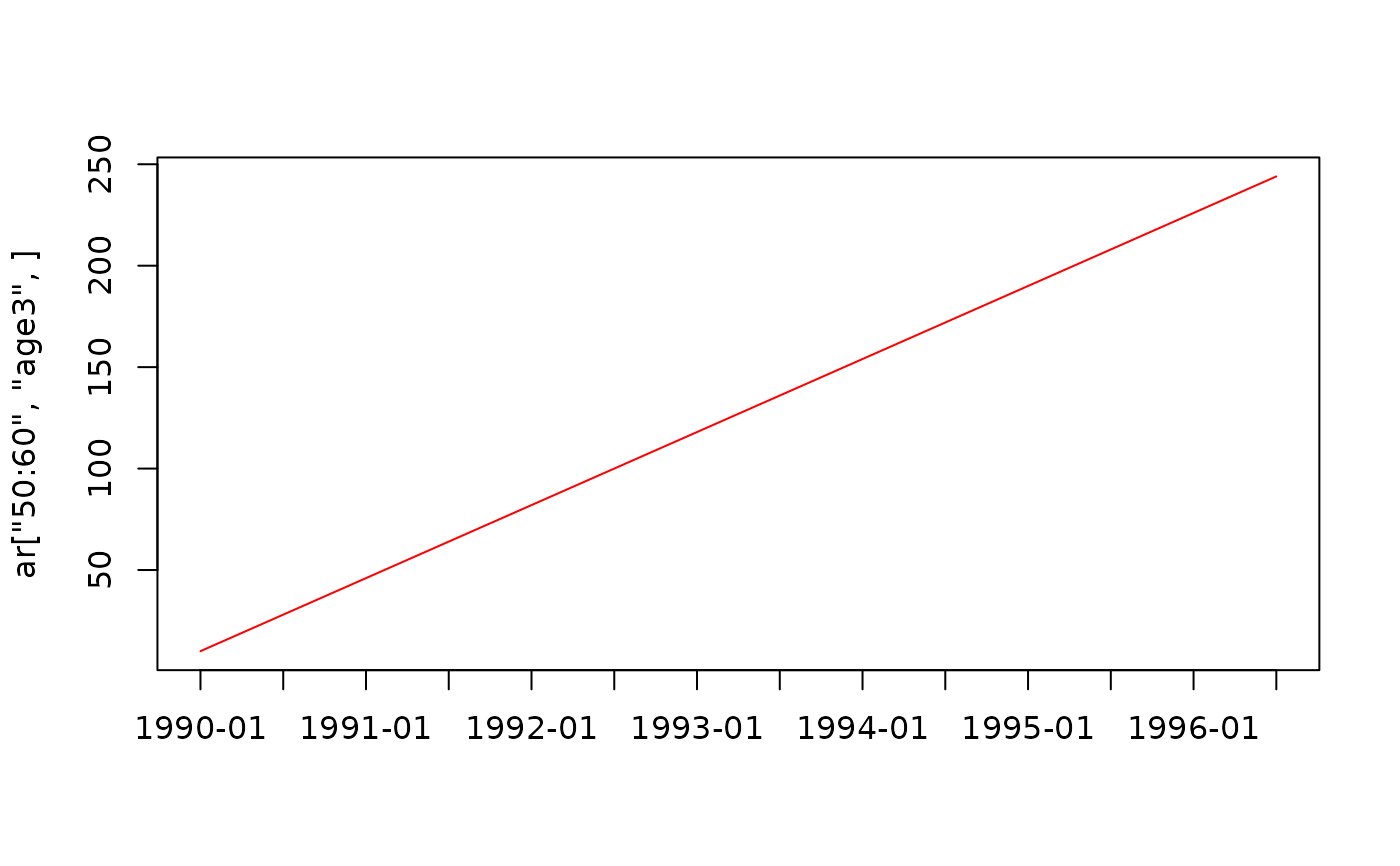
g3_array_plot will plot the contents of an array, for arrays with 2 dimensions or less.

Value

An array, filtered by ... and aggregated by margins.

If ar was a list, a list of filtered/aggregated arrays

Examples

# Generate an array to test with
dn <- list(
    length = c("50:60", "60:70", "70:Inf"),
    age = paste0("age", 0:5),
    time = paste0(rep(1990:1996, each = 2), c("-01", "-02")) )
ar <- array(
    seq_len(prod(sapply(dn, length))),
    dim = sapply(dn, length),
    dimnames = dn)
ar[,,"1994-02", drop = FALSE]
#> , , time = 1994-02
#> 
#>         age
#> length   age0 age1 age2 age3 age4 age5
#>   50:60   163  166  169  172  175  178
#>   60:70   164  167  170  173  176  179
#>   70:Inf  165  168  171  174  177  180
#> 
g3_array_plot(ar[,,"1994-02"])

g3_array_plot(ar["50:60","age3",])


# Generate by-year report for ages 2..4
g3_array_agg(ar, c('age', 'year'), age = 2:4)
#>       year
#> age    1990 1991 1992 1993 1994 1995 1996
#>   age2  102  318  534  750  966 1182 1398
#>   age3  120  336  552  768  984 1200 1416
#>   age4  138  354  570  786 1002 1218 1434

# ...for only step 1
g3_array_agg(ar, c('age', 'year'), age = 2:4, step = 1)
#>       year
#> age    1990 1991 1992 1993 1994 1995 1996
#>   age2   24  132  240  348  456  564  672
#>   age3   33  141  249  357  465  573  681
#>   age4   42  150  258  366  474  582  690

# Report on smallest length group, for each timestep
g3_array_agg(ar, c('length', 'time'), length = 55)
#>        time
#> length  1990-01 1990-02 1991-01 1991-02 1992-01 1992-02 1993-01 1993-02 1994-01
#>   50:60      51     159     267     375     483     591     699     807     915
#>        time
#> length  1994-02 1995-01 1995-02 1996-01 1996-02
#>   50:60    1023    1131    1239    1347    1455
# Use midlen as the dimension name
g3_array_agg(ar, c('length', 'time'), length = 55, opt_length_midlen = TRUE)
#>       time
#> length 1990-01 1990-02 1991-01 1991-02 1992-01 1992-02 1993-01 1993-02 1994-01
#>     55      51     159     267     375     483     591     699     807     915
#>       time
#> length 1994-02 1995-01 1995-02 1996-01 1996-02
#>     55    1023    1131    1239    1347    1455

# Combine 2 arrays with disjoint age ranges into one list
g3_array_combine(list(
    g3_array_agg(ar, c('age', 'year'), age = 2:4),
    g3_array_agg(ar / 1000, c('age', 'year'), age = 3:5) ))
#>       year
#> age       1990    1991    1992    1993     1994     1995     1996
#>   age2 102.000 318.000 534.000 750.000  966.000 1182.000 1398.000
#>   age3 120.120 336.336 552.552 768.768  984.984 1201.200 1417.416
#>   age4 138.138 354.354 570.570 786.786 1003.002 1219.218 1435.434
#>   age5   0.156   0.372   0.588   0.804    1.020    1.236    1.452

# We can aggregate lists of arrays, applying the same options for each
list(a = ar, b = ar * 10) |> g3_array_agg(c('year', 'age'), length = 55)
#> $a
#>       year
#> age    1990 1991 1992 1993 1994 1995 1996
#>   age0   20   92  164  236  308  380  452
#>   age1   26   98  170  242  314  386  458
#>   age2   32  104  176  248  320  392  464
#>   age3   38  110  182  254  326  398  470
#>   age4   44  116  188  260  332  404  476
#>   age5   50  122  194  266  338  410  482
#> 
#> $b
#>       year
#> age    1990 1991 1992 1993 1994 1995 1996
#>   age0  200  920 1640 2360 3080 3800 4520
#>   age1  260  980 1700 2420 3140 3860 4580
#>   age2  320 1040 1760 2480 3200 3920 4640
#>   age3  380 1100 1820 2540 3260 3980 4700
#>   age4  440 1160 1880 2600 3320 4040 4760
#>   age5  500 1220 1940 2660 3380 4100 4820
#> 

# We can aggregate then combine
list(a = ar, b = ar * 10) |>
     g3_array_agg(c('year', 'age'), length = 55) |> g3_array_combine()
#>       year
#> age    1990 1991 1992 1993 1994 1995 1996
#>   age0  220 1012 1804 2596 3388 4180 4972
#>   age1  286 1078 1870 2662 3454 4246 5038
#>   age2  352 1144 1936 2728 3520 4312 5104
#>   age3  418 1210 2002 2794 3586 4378 5170
#>   age4  484 1276 2068 2860 3652 4444 5236
#>   age5  550 1342 2134 2926 3718 4510 5302